One line, one elevation
A contour connects equal heights. Travel along a 1100 m contour and the modeled elevation stays 1100 m, even when the line curves. It is an imaginary line, not a path.
Explore the hill study ↗Field school / 01 · Topography
A line on a map becomes a fold in the landscape. Follow the contours, turn the terrain, and learn to see what lies between.
The reading guide
Work in any order. These lessons and the field plates below are the complete static alternative.
A contour connects equal heights. Travel along a 1100 m contour and the modeled elevation stays 1100 m, even when the line curves. It is an imaginary line, not a path.
Explore the hill study ↗The interval is a vertical difference, in metres here. At 20 m, successive lines can be 1080, 1100 and 1120 m. Our heavier index lines mark every fifth interval. A smaller interval adds lines without adding terrain detail.
Explore the slope study ↗On this hill, labels rise inward. Closed contours can also surround a depression; its elevations fall inward, often with short inward ticks called hachures. A loop alone does not prove a summit.
Explore the hill study ↗Compare lines on the same map and at the same interval. Tight spacing means a steep slope; wide spacing means a gentle one. Grade = vertical rise ÷ horizontal run × 100%. A 20 m rise over 100 m is 20%, about 11.3°, not 20°.
Explore the slope study ↗In the teaching valley, contours bend toward higher ground at the valley floor. The north–south profile confirms the direction. Water would tend downhill across the contours; this diagram maps no actual stream.
Explore the valley study ↗The ridge has high ground along its spine and lower flanks. Its contour nose points downhill. Similar-looking bends need elevation labels and surrounding context before you name the landform.
Explore the ridge study ↗Pass a section through the same center in two perpendicular directions. One profile makes a hollow; the other makes a crest. At the exact saddle elevation, a level set can touch itself. Our fixed triangulation makes that special case explicit.
Explore the saddle study ↗Aspect is the direction of steepest descent: 0° north, 90° east, 180° south, 270° west. This kit uses grid north, not a magnetic compass bearing. Aspect at a perfectly flat or symmetric critical point is undefined.
Explore the slope study ↗A–B is a straight horizontal sampling line. The chart plots distance along it against elevation. Move the section and you sample different ground. It is not a hiking route; no path length or trail difficulty follows from the section.
Explore the bryce study ↗At 3× vertical exaggeration, a 20 m height difference is drawn three times as tall relative to horizontal distance. The stored heights, contour interval and calculated slope stay unchanged. Return to 1× before judging shape; even then, a sampled grid omits small and hidden features.
Explore the bryce study ↗The field plate library
Twelve standalone vector diagrams, with both central profiles and sample tables. Open a plate at full size, or open the print edition for the complete guide.
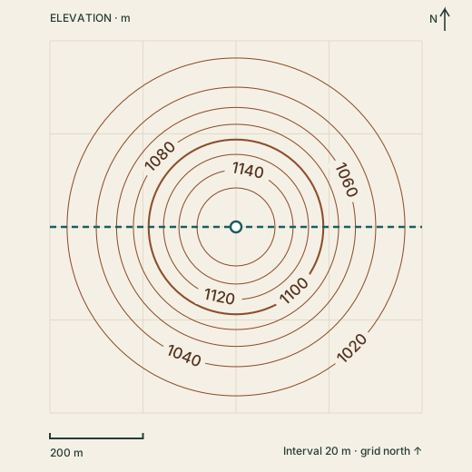
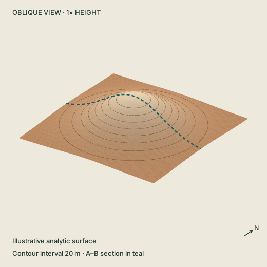
A circular hill rises from about 1001 m at the corners to 1180 m at its center. The central west–east profile rises and falls symmetrically.
Both charts use equal horizontal and vertical scale (1×). The plate’s dashed line shows west–east; north–south crosses it at the center.
| Distance from A | West–east | North–south |
|---|---|---|
| 0 m | 1012.5 | 1012.5 |
| 200 m | 1092.4 | 1092.4 |
| 400 m | 1180.0 | 1180.0 |
| 600 m | 1092.4 | 1092.4 |
| 800 m | 1012.5 | 1012.5 |
These labeled rings rise inward toward a summit. Closed rings alone are not enough: descending labels or inward hachures can identify a depression.
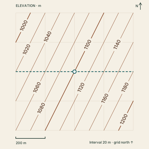
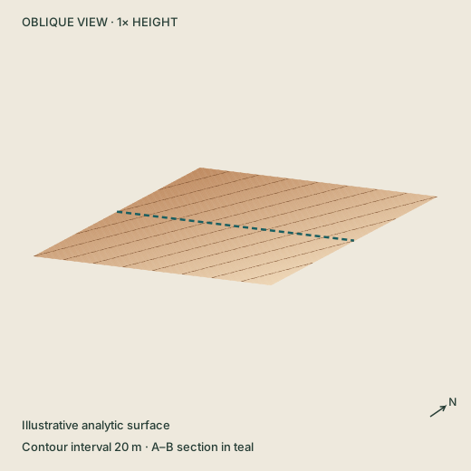
Parallel, evenly spaced contours cross a tilted plane. Elevation increases eastward and southward. The west–east center profile rises from 1020 m to 1180 m.
Both charts use equal horizontal and vertical scale (1×). The plate’s dashed line shows west–east; north–south crosses it at the center.
| Distance from A | West–east | North–south |
|---|---|---|
| 0 m | 1020.0 | 1060.0 |
| 200 m | 1060.0 | 1080.0 |
| 400 m | 1100.0 | 1100.0 |
| 600 m | 1140.0 | 1120.0 |
| 800 m | 1180.0 | 1140.0 |
The surface is unchanged. Here each 100 m east adds 20 m of elevation; each 100 m south adds 10 m. The steepest slope is about 12.6° (22.4%), down toward 297° from grid north.
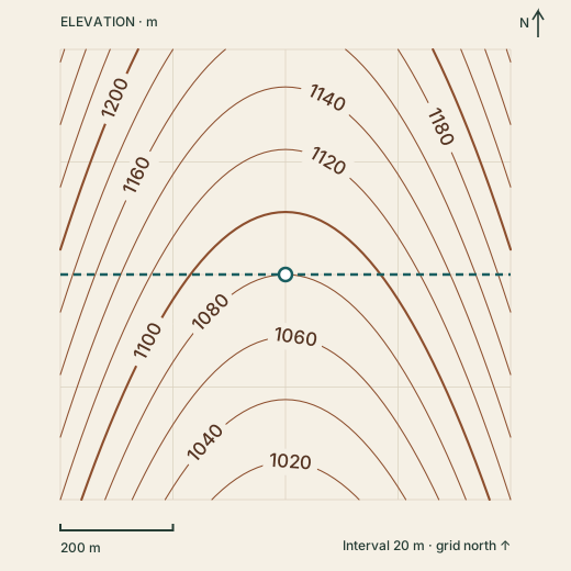
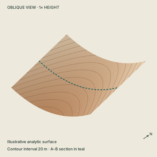
Rounded V-shaped contours point north. Each side is higher than the valley floor. A north–south profile along the center falls from 1152 m to 1008 m.
Both charts use equal horizontal and vertical scale (1×). The plate’s dashed line shows west–east; north–south crosses it at the center.
| Distance from A | West–east | North–south |
|---|---|---|
| 0 m | 1192.0 | 1152.0 |
| 200 m | 1108.0 | 1116.0 |
| 400 m | 1080.0 | 1080.0 |
| 600 m | 1108.0 | 1044.0 |
| 800 m | 1192.0 | 1008.0 |
In this valley the contour bends point north, toward higher ground. A contour is not a stream: the valley floor descends southward across the contour lines.
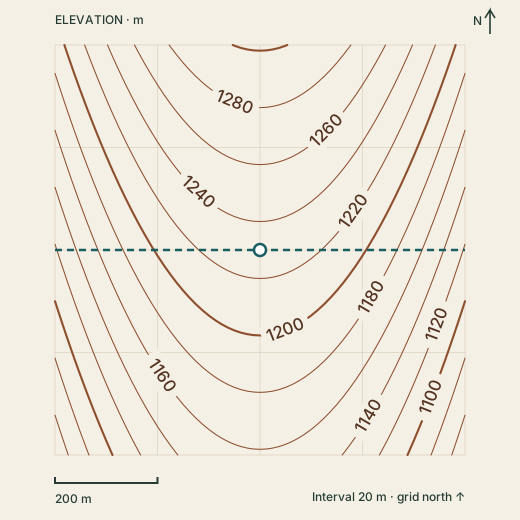
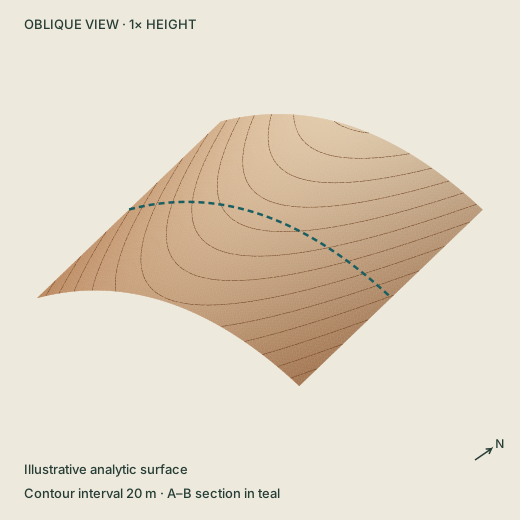
Contours bow south around a crest. The center is high compared with its east and west flanks. The central west–east profile rises to 1230 m and falls again.
Both charts use equal horizontal and vertical scale (1×). The plate’s dashed line shows west–east; north–south crosses it at the center.
| Distance from A | West–east | North–south |
|---|---|---|
| 0 m | 1118.0 | 1302.0 |
| 200 m | 1202.0 | 1266.0 |
| 400 m | 1230.0 | 1230.0 |
| 600 m | 1202.0 | 1194.0 |
| 800 m | 1118.0 | 1158.0 |
This ridge nose points south, downhill. The crest is higher than the land on either side. Read the labels to distinguish a ridge from a valley.
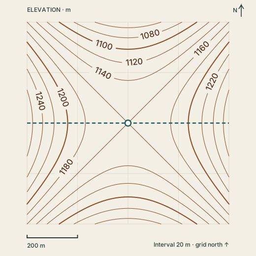
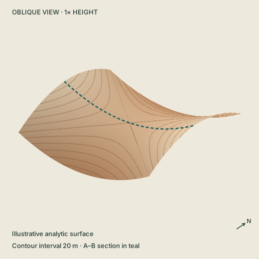
The center is a low point on a west–east section and a high point on a north–south section. The saddle has no single downhill aspect exactly at its center.
Both charts use equal horizontal and vertical scale (1×). The plate’s dashed line shows west–east; north–south crosses it at the center.
| Distance from A | West–east | North–south |
|---|---|---|
| 0 m | 1272.0 | 1048.0 |
| 200 m | 1188.0 | 1132.0 |
| 400 m | 1160.0 | 1160.0 |
| 600 m | 1188.0 | 1132.0 |
| 800 m | 1272.0 | 1048.0 |
At 1160 m the center is lower than its east and west shoulders, but higher than the north and south approaches. The exact critical-level contour touches here; real map generalization can hide this special case.
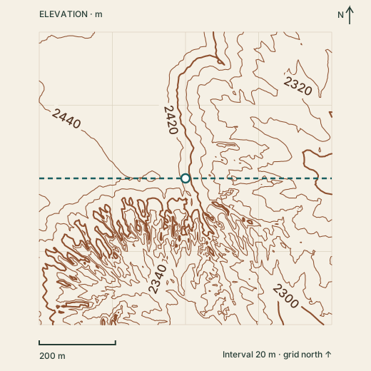
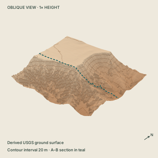
An irregular plateau edge gives way to steep, closely spaced contours and lower branching terrain. Heights in this crop range from 2286.5 m to 2468.1 m NAVD88. The cut boundary is editorial.
Both charts use equal horizontal and vertical scale (1×). The plate’s dashed line shows west–east; north–south crosses it at the center.
| Distance from A | West–east | North–south |
|---|---|---|
| 0 m | 2456.7 | 2430.7 |
| 192 m | 2442.7 | 2385.2 |
| 384 m | 2413.5 | 2413.5 |
| 576 m | 2334.4 | 2357.0 |
| 768 m | 2292.5 | 2309.0 |
This 768 m square comes from an existing USGS bare-earth terrain derivative, sampled every 8 m. Thin fins and steep breaks can be simplified. It cannot recover hidden rock faces, establish a route or replace a ground-level scan.
Read the evidence, too
The first five surfaces are mathematical illustrations. The Bryce study is derived from a copied USGS bare-earth terrain grid: a 768 m square sampled every 8 m, with heights retained in NAVD88 metres. The original DEM was recorded as 1 m resolution; the copied regional record does not identify an individual source tile or acquisition date. These lines do not establish trails, rock stability, survey positions or present-day conditions.
Map services and data available from U.S. Geological Survey, National Geospatial Program. Contour School’s diagrams, lighting, code and explanations are original. No source photographs or third-party map images are included. The terrain is not a ground-level scan of Thor’s Hammer.
References checked October 2, 2026. Read equations, data lineage & limitations · Structured lesson & asset catalogue